Visualizing Softmax

Introduction

I have been faced with several situations where visualizing the output of a trained classifier has helped explain some interesting behaviors that are present within learned representations. I want to share a simple technique to visualize outputs for SoftMax-based classifiers. As an example, I will walk through the process of visualizing and animating the effects of Temperature Scaling, which is a simple and useful technique for knowledge transfer [1] and model calibration [2][3][4].

Softmax

For deep neural networks (DNN) the representation is related to the construction of the optimization objective. In the case of DNN image classifiers the most common objective is to minimize the softmax cross entropy between the model output, \(\boldsymbol{v}\in\mathbb{R}^k\) and a one-hot target, $\boldsymbol{y}$. In order to compute the cross entropy, \(\boldsymbol{v}\) must first be projected onto a simplex to become "probability-like". \( \boldsymbol{\sigma}:\mathbb{R}^k\rightarrow\boldsymbol{\Delta}^{k-1}\\ \) The resulting vector, $\boldsymbol{q}\in\boldsymbol{\Delta}^{k-1}$, is the output of the softmax operation, $\boldsymbol{\sigma}$. To simplify notation, let \(\mathbf{e}^{\boldsymbol{v}}= \left(\begin{smallmatrix}e^{v_0}& e^{v_1}&\dots&e^{v_{k-1}}\end{smallmatrix}\right)\).

\[ \boldsymbol{q} = \frac{\mathbf{e}^{\boldsymbol{v}}}{\sum^{k-1}_{i=0} e^{v_i}} \]

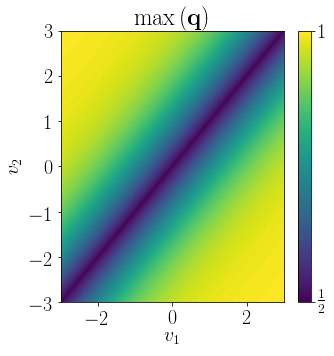
Here's a visualization of SoftMax for the $k=2$ case.

It is then possible to assign a confidence, $c$, to a prediction by selecting the maximum component $c = \max(\boldsymbol{q})$.

Visualizing Softmax at higher dimensions

My research mostly concerns classification or detection problems for images, which tends to involve more than 2 classes. In order to visualize the behavior of softmax at $k>2$ we want to stay away from techniques that rely on the data directly (t-SNE, UMAP, PCA, etc.) and instead use a technique that can capture the macro behaviors in the representation space by prior construction. Doing this is likely not without loss of information, because data-driven methods seek to find some transformation that preserves information.

The first thing to do is to inspect the space to which softmax projects $\boldsymbol v$, the $(k-1)$-simplex $\boldsymbol{\Delta}^{k-1}$, to better understand some useful properties for projection. Loosely defined, a simplex is the generalization of the triangle. In the case of the triangle it would be a 2-simplex. Below I generated a tikz visualization of the 0 to 3 simplexes:

Take note of the graphical structure of simplexes as it will come into play in later discussion. Now for a more formal definition of a simplex with regard to our softmax projection, \(\boldsymbol{\sigma}:\mathbb{R}^k\rightarrow\boldsymbol{\Delta}^{k-1}\).

As we previously defined, $\mathbf{q}$ is the resulting projected vector that follows the definition,

\[ \{\mathbf{q}\in\mathbb{R}^k:\sum_i q_i=1, q_i\geq 0, i=0,\dots,k-1\}, \]

which allows it to be used as a probability distribution. The fact that all of the information is projected into the positive orthant is also useful as now every component, $q_i\in\mathbf{q}$, can be used to form a star-like graph about the origin:

This projection is just a way to view these components in such a way at arbitrary dimensions such that the angle between each when projected is equal. And thus, forevermore throughout this post, such a technique shall be called the Equiradial Projection (EqR).

Where the angle between components is

\[ \theta_i = \frac{2\pi (i+0.5)}{k}, \quad i=\{0,\dots,k-1\} \]

and the projection matrix is

\[ \boldsymbol{T} = \begin{pmatrix} \sin(\theta_0) &\sin(\theta_1) &\cdots & \sin(\theta_{k-1}) \\ \cos(\theta_0) &\cos(\theta_1) &\cdots & \cos(\theta_{k-1}) \\ \end{pmatrix},\\ \]

making $\boldsymbol{T}\boldsymbol{q}$ just the weighted average of the projected components. This is where distortions and loss of information come into play. The derivation of the projection is based on the assumption that the space is star-like, meaning that each component occurs in isolation. We know that this is in fact not the case most of the time as $\boldsymbol{q}$ by definition is a probability distribution making all but $k$ cases violate this assumption.

Now that this loss of information and distortion is acknowledged we need to discuss rotation. When the order of the components changes in the projection the view is just rotating about another component orthoganally. This can provide some limited ability to minimize distortion by placing the most dependent subsets of components adjacent.

Temperature Scaling

Hinton et al. [1] introduced technique used for knowledge transfer called "Knowledge Distillation" that increases the temperature, $T$, on $\boldsymbol{v}$ in order to generate a softer representation out of softmax. In [2], Guo et al, refers to the same technique as "Temperature Scaling":

\[ \boldsymbol{q}_{temp} = \frac{\mathbf{e}^{\boldsymbol{v}/T}}{\sum^{k-1}_{i=0} e^{v_i/T}} , \qquad T\in\mathbb{R}^+ \]

This simple technique has proven to be incredibly useful beyond the initial proposed use in knowledge transfer. Guo et al. demonstrated its utility in calibrating deep models for image classification. In both [3][4], they use temperature scaling to great effect in detecting out-of-distribution samples.

And without further ado, let's visualize temperature scaled softmax outputs in arbitrary dimensions!

For $\boldsymbol{v}$, I just generated random vectors in the desired dimension and visualized the projection at a variation of $T$. Each vector is colored according to the confidence at that location on the projection.

Citations

1: G. E. Hinton, O. Vinyals, and J. Dean, “Distilling the knowledge in a neural network,” ArXiv, vol. abs/1503.02531, 2015.

2: C. Guo, G. Pleiss, Y. Sun, and K. Q. Weinberger, “On calibration of modern neural networks,” in Proceedings of the 34th international conference on machine learning-volume 70, 2017, pp. 1321–1330.

3: K. Lee, H. Lee, K. Lee, and J. Shin, “Training confidence-calibrated classifiers for detecting out-of-distribution samples,” in International conference on learning representations, 2018.

4: S. Liang, Y. Li, and R. Srikant, “Enhancing the reliability of out-of-distribution image detection in neural networks,” in International conference on learning representations, 2018.