Learning to segment CIFAR10

Import Important Things

import torch
from torch import nn
import torch.nn.functional as F
from torch.utils.data import DataLoader
from torchvision import transforms
from torchvision.models import resnet18
from torchvision.datasets import CIFAR10
from tqdm import tqdm_notebook as tqdm
from torchvision.utils import save_image, make_grid
from matplotlib import pyplot as plt
from matplotlib.colors import hsv_to_rgb
from matplotlib.image import BboxImage
from matplotlib.transforms import Bbox, TransformedBbox
import numpy as np
from IPython import display
import requests
from io import BytesIO
from PIL import Image
from PIL import Image, ImageSequence
from IPython.display import HTML
import warnings
from matplotlib import rc
import gc
import matplotlib
matplotlib.rcParams['pdf.fonttype'] = 42
matplotlib.rcParams['ps.fonttype'] = 42
gc.enable()
plt.ioff()

Initialize the tiny model from ResNet18

I am replacing the first 7x7 conv stride of 4 with a 3x3 convolution kernel with stride of 1 and replacing maxpool with upsample. This keeps the spatial features from being downsampled too quickly as the forward pass propagates. The linear layer is replaced with a "pixelwise linear layer", or a 1x1 convolution with stride of 1. This can be simply thought of as projecting a 1x512 vector (pixel) with a 512x10 matrix (1x1 conv). Notice that there is no operation that performs a spatial aggregation so what we have left is a 10x32x32 tensor after the final upsample. This can be used the same way as a semantic segmentation output, which we can also aggregate spatially and optimize using image level labels.

num_classes = 10
resnet = resnet18(pretrained=True)
resnet.conv1 = nn.Conv2d(3,64,3,stride=1,padding=1)
resnet_ = list(resnet.children())[:-2]
resnet_[3] = nn.Upsample(scale_factor=2, mode='bilinear', align_corners=False)
classifier = nn.Conv2d(512,num_classes,1)
torch.nn.init.kaiming_normal_(classifier.weight)
resnet_.append(classifier)
resnet_.append(nn.Upsample(size=32, mode='bilinear', align_corners=False))
tiny_resnet = nn.Sequential(*resnet_)

Define Attention

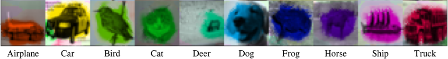
In short, I'm going to just define 0 as the threshold in the logit (pre-softmax space). By selecting the largest component of the logit vector and then running it through sigmoid we can get a value with a support from 0 to 1, which is useful for inspecting the "attention" of the model.

def attention(x):
    return torch.sigmoid(torch.logsumexp(x,1, keepdim=True))

CIFAR10 dataset

This dataset is so convenient for demonstrating so many things. There are much more impressive demonstrations of weak segmentation, but all of this can be accomplished in a jupyter notebook so here we go!

transform_train = transforms.Compose([
    transforms.RandomCrop(32, padding=8),
    transforms.RandomHorizontalFlip(),
    transforms.ToTensor(),
    transforms.Normalize((0.4914, 0.4822, 0.4465), (0.2023, 0.1994, 0.2010)),
])

transform_test = transforms.Compose([
    transforms.ToTensor(),
    transforms.Normalize((0.4914, 0.4822, 0.4465), (0.2023, 0.1994, 0.2010)),
])

trainset = CIFAR10(root='.', train=True, download=True, transform=transform_train)
train_iter = DataLoader(trainset, batch_size=128, shuffle=True, num_workers=16, pin_memory=True, drop_last=True)

testset = CIFAR10(root='.', train=False, download=True, transform=transform_test)
test_iter = DataLoader(testset, batch_size=100, shuffle=False, num_workers=16, pin_memory=True)

classes = ('plane', 'car', 'bird', 'cat', 'deer', 'dog', 'frog', 'horse', 'ship', 'truck')

Files already downloaded and verified
Files already downloaded and verified

Train and Visualize

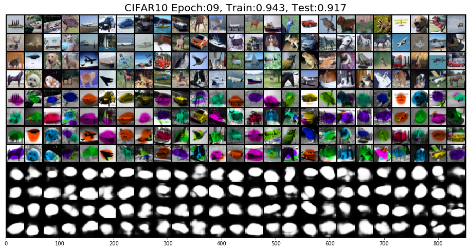
The key take aways from the below code is that the objective for optimization is Binary Cross Entropy and the model's spatial aggregation is accomplished with a smooth-max operation. This means after aggregation the vector is optimized to be a set of 10 binary detectors, which is in contrast to the most popular method of characterization: softmax cross entropy, which encourages each pixel to select only one. When combined with the aforementioned attention operation we can forego aggregation and directly inspect exactly what the model uses to make a decision!

model = nn.DataParallel(tiny_resnet).cuda()
num_epochs = 10
criterion = nn.BCEWithLogitsLoss()
optimizer = torch.optim.SGD(model.parameters(), lr = 0.05, momentum=0.9, weight_decay=1e-4)
lr_scheduler = torch.optim.lr_scheduler.CosineAnnealingLR(optimizer,78,eta_min=0.001)

losses = []
acces = []
v_losses = []
v_acces = []
for epoch in tqdm(range(num_epochs)):
    epoch_loss = 0.0
    acc = 0.0
    var = 0.0
    model.train()
    train_pbar = train_iter
    for i, (x, _label) in enumerate(train_pbar):
        x = x.cuda()
        _label = _label.cuda()
        label = F.one_hot(_label).float()
        seg_out = model(x)
        
        attn = attention(seg_out)
        # Smooth Max Aggregation
        logit = torch.log(torch.exp(seg_out*0.5).mean((-2,-1)))*2
        loss = criterion(logit, label)
        optimizer.zero_grad()
        loss.backward()
        optimizer.step()
        lr_scheduler.step()
        epoch_loss += loss.item()
        acc += (logit.argmax(-1)==_label).sum()
        #train_pbar.set_description('Accuracy: {:.3f}%'.format(100*(logit.argmax(-1)==_label).float().mean()))
        
    avg_loss = epoch_loss / (i + 1)
    losses.append(avg_loss)
    avg_acc = acc.cpu().detach().numpy() / (len(trainset))
    acces.append(avg_acc)
    model.eval()
    epoch_loss = 0.0
    acc = 0.0
    num_seen = 0
    
    test_pbar = tqdm(test_iter)
    for i, (x, _label) in enumerate(test_pbar):
        x = x.cuda()
        _label = _label.cuda()
        label = F.one_hot(_label).float()
        seg_out = model(x)
        attn = attention(seg_out)
        logit = torch.log(torch.exp(seg_out*0.5).mean((-2,-1)))*2
        loss = criterion(logit, label)
        epoch_loss += loss.item()
        acc += (logit.argmax(-1)==_label).sum()
        num_seen += label.size(0)
        test_pbar.set_description('Accuracy: {:.3f}%'.format(100*(acc.float()/num_seen)))
    
    avg_loss_val = epoch_loss / (i + 1)
    v_losses.append(avg_loss_val)
    avg_acc_val = acc.cpu().detach().numpy() / (len(testset))
    v_acces.append(avg_acc_val)
    plt.close('all')

    conf = torch.max(nn.functional.softmax(seg_out, dim=1), dim=1)[0]
    hue = (torch.argmax(seg_out, dim=1).float() + 0.5)/10
    x -= x.min()
    x /= x.max()
    gs_im = x.mean(1)
    gs_mean = gs_im.mean()
    gs_min = gs_im.min()
    gs_max = torch.max((gs_im-gs_min))
    gs_im = (gs_im - gs_min)/gs_max
    hsv_im = torch.stack((hue.float(), attn.squeeze().float(), gs_im.float()), -1)
    im = hsv_to_rgb(hsv_im.cpu().detach().numpy())
    ex = make_grid(torch.tensor(im).permute(0,3,1,2), normalize=True, nrow=25)
    attns = make_grid(attn, normalize=False, nrow=25)
    attns = attns.cpu().detach()
    inputs = make_grid(x, normalize=True, nrow=25).cpu().detach()
    display.clear_output(wait=True)
    plt.figure(figsize=(20,8))
    plt.imshow(np.concatenate((inputs.numpy().transpose(1,2,0),ex.numpy().transpose(1,2,0), attns.numpy().transpose(1,2,0)), axis=0))
    #plt.xticks(np.linspace(18,324,10), classes)
    #plt.xticks(fontsize=20) 
    plt.yticks([])
    plt.title('CIFAR10 Epoch:{:02d}, Train:{:.3f}, Test:{:.3f}'.format(epoch, avg_acc, avg_acc_val), fontsize=20)
    display.display(plt.gcf())
    fig, ax = plt.subplots(1,2, figsize=(20,8))
    ax[0].set_title('Crossentropy')
    ax[0].plot(losses, label='Train')
    ax[0].plot(v_losses, label='CIFAR10 Test')
    ax[0].legend()
    ax[1].set_title('Accuracy')
    ax[1].plot(acces, label='Train')
    ax[1].plot(v_acces, label='CIFAR10 Test')
    ax[1].legend()
    display.display(plt.gcf())
    

I only trained it for 10 epochs here and get a passable performance, which does improve if it goes further. I stopped it to leave some of the mixed decisions the model is making. Declaring success here is premature for calling this as a great method for weak segmentation, but it does show exactly what the model considers spatially for every decision it makes. Once more, the model only uses values that are very positive thus saturating sigmoid to make a decision, by combining the argmax with the attention operation defined we can get the below visualization. The examples that show multiple colors are examples that share features with other classes, i.e. the birds and airplanes, deer and horses, cars and trucks. Now if there were only a method for looking at where all the pixels project into the learned space all at once!

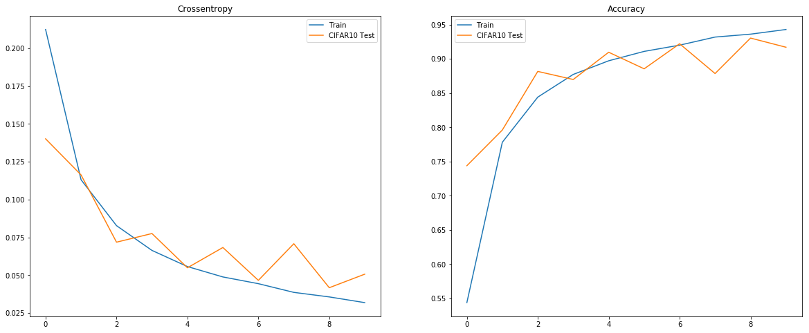
Though not absolutely necessary here's what the numbers look like during training.