Blackjack Simulator
I worked with Gukyeong Kwon and Jinsol Lee on this project for our Convex Optimization course. It was a neat project that really hits home that even if you can count cards perfectly…the deck isn’t stacked in your favor. If you want to try it the code is linked above or if you want to run blackjacksim directly install it with:
pip3 install git+https://github.com/charlieLehman/blackjacksim
Tools
from sklearn.metrics import confusion_matrix
from sklearn.utils.multiclass import unique_labels
import matplotlib
from mpl_toolkits.axes_grid1 import make_axes_locatable
%matplotlib inline
from matplotlib import pyplot as plt

def plot_confusion_matrix(y_true, y_pred, classes,
                          normalize=False,
                          title=None,
                          cmap=plt.cm.Blues,
                         **kwargs):
    """
    This function prints and plots the confusion matrix.
    Normalization can be applied by setting `normalize=True`.
    """
    if not title:
        if normalize:
            title = 'Normalized confusion matrix'
        else:
            title = 'Confusion matrix, without normalization'

    # Compute confusion matrix
    cm = confusion_matrix(y_true, y_pred)
    # Only use the labels that appear in the data
    #classes = classes[unique_labels(y_true, y_pred)]
    if normalize:
        cm = cm.astype('float') / cm.sum(axis=1)[:, np.newaxis]
        print("Normalized confusion matrix")
    else:
        print('Confusion matrix, without normalization')

    print(cm)

    fig, ax = plt.subplots(**kwargs)
    im = ax.imshow(cm, interpolation='nearest', cmap=cmap)
    divider = make_axes_locatable(ax)
    cax = divider.append_axes("right", size="5%", pad=0.05)
    ax.figure.colorbar(im, cax=cax)
    # We want to show all ticks...
    ax.set(xticks=np.arange(cm.shape[1]),
           yticks=np.arange(cm.shape[0]),
           # ... and label them with the respective list entries
           xticklabels=classes, yticklabels=classes,
           ylabel='True label',
           xlabel='Predicted label')

    # Rotate the tick labels and set their alignment.
    plt.setp(ax.get_xticklabels(), rotation=45, ha="right",
             rotation_mode="anchor")

    # Loop over data dimensions and create text annotations.
    fmt = '.2f' if normalize else 'd'
    thresh = cm.max() / 2.
    for i in range(cm.shape[0]):
        for j in range(cm.shape[1]):
            ax.text(j, i, format(cm[i, j], fmt),
                    ha="center", va="center",
                    color="white" if cm[i, j] > thresh else "black")


    fig.tight_layout()
    return ax
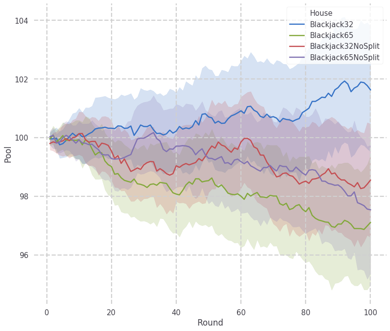
Comparison of House Rules
from blackjacksim.simulations import Game
from blackjacksim.entities import Shoe
import matplotlib
%matplotlib inline
from tqdm import tnrange
from tqdm import tqdm_notebook as tqdm
from matplotlib import pyplot as plt
import seaborn as sns
import pandas as pd
from jupyterthemes import jtplot
jtplot.style(context='poster', fscale=1.4, spines=False, gridlines='--')

from blackjacksim.data import DefaultGameConfig
_def_conf = DefaultGameConfig()
def config(house_rules):
    _def_conf['house']['class'] = house_rules
    return _def_conf

try:
    df = df
except:
    df = None

pbar = tqdm(['Blackjack32', 'Blackjack65', 'Blackjack32NoSplit', 'Blackjack65NoSplit'])
trials = 100
rounds = 100
for house in pbar:
    for i in range(trials):
        pbar.set_description("{} {:04d}/{:04d}: ".format(house,i,trials-1))
        g = Game(config(house))
        for _ in range(rounds):
            g.round()
        if df is None:
            df = g.data
        else:
            df = pd.concat([df,g.data])

sns.lineplot(x='Round', y='Pool', hue='House', data=df)
plt.show()
HBox(children=(IntProgress(value=0, max=4), HTML(value='')))
Modeling Action Strategy
Build board state matrix A and action vector b
from blackjacksim.entities import Deck, Hand
from blackjacksim.strategies import basic
import itertools
import numpy as np
import pandas as pd

action_to_class = {'Hit':[1,0,0,0],'Stand':[0,1,0,0],'Split':[0,0,1,0],'Double':[0.0,0,0,1]}

hands = [Hand(h) for h in itertools.product(Deck(),Deck())]
dups = Deck()

t = []
for hand, dup  in itertools.product(hands, dups):
    tup = tuple(c.value for c in (*hand,dup))
    c = (tup, basic(hand,dup))
    if c not in t:
        t.append(c)
print(len(t))
A = []
b = []
for  a, _b in t:
    A.append(a)
    b.append(action_to_class[_b])

A = np.stack(A)
b = np.array(b)
1001
Solve Least Squares
import seaborn as sns
from jupyterthemes import jtplot
jtplot.style(context='paper', fscale=1.4, spines=False, gridlines='')
A_ = np.concatenate([A, np.ones((A.shape[0],1))],1)
Ai = np.linalg.pinv(A_)
x = Ai@b
out = A_@x
pred = np.argmax(out,1)
lab = np.argmax(b,1)
lab_to_class = list(action_to_class.keys())
l2c = lambda x: lab_to_class[x]
df = pd.DataFrame({'Prediction':pred, 'Label':lab,'HandSum':A[:,0:-1].sum(1), 'Hand':[a[0:-1] for a in A], 'Up Card':[a[-1] for a in A]})
df['Label Name'] = df.Label.apply(l2c)
df['Prediction Name'] = df.Prediction.apply(l2c)
df['Correct'] = df.Prediction == df.Label
# Plot normalized confusion matrix
classes = list(action_to_class.keys())
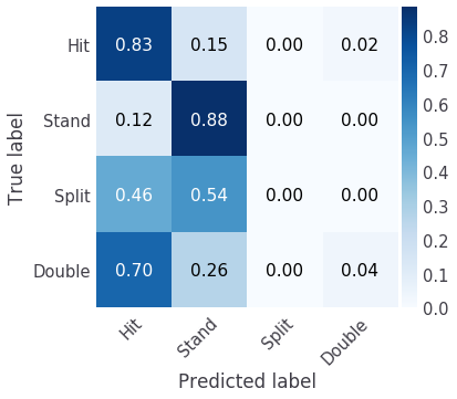
print('Accuracy: {:.2f}%\n'.format(df.Correct.mean()*100))
plot_confusion_matrix(lab, pred, classes=classes, normalize=True, title=' ', figsize=(6,6))
plt.show()
Accuracy: 65.53%

Normalized confusion matrix
[[0.82826087 0.14782609 0.         0.02391304]
 [0.11551155 0.88448845 0.         0.        ]
 [0.45833333 0.54166667 0.         0.        ]
 [0.7        0.26315789 0.         0.03684211]]
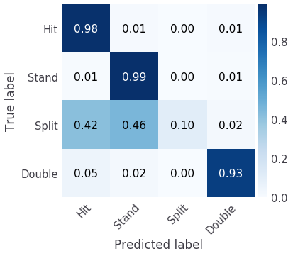
Solve SVM with RBF kernel
from sklearn.svm import SVC
clf = SVC(gamma='auto', probability=True)
label = b.argmax(1)
clf.fit(A,label)
print(clf.score(A,label))
pred = clf.predict(A)

vals = clf.decision_function(A)
probs = clf.predict_proba(A)

classes = list(action_to_class.keys())
plot_confusion_matrix(label, pred, classes=classes, normalize=True, title=' ', figsize=(6,6))
plt.show()
0.932067932067932
Normalized confusion matrix
[[0.9826087  0.00869565 0.         0.00869565]
 [0.00660066 0.98679868 0.         0.00660066]
 [0.41666667 0.45833333 0.10416667 0.02083333]
 [0.04736842 0.02105263 0.         0.93157895]]
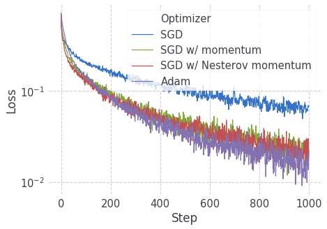
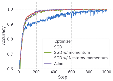
Comparison of Optimizers for a Deep Model
Train
from blackjacksim.entities import Deck, Hand
from blackjacksim.strategies import basic
import itertools
import numpy as np
import pandas as pd
import torch
from torch import nn
from tqdm import tnrange


# Build A (Hand and Dealer's Up Card) and b (basic strategy Action)
action_to_class = {'Hit':[1,0,0,0],'Stand':[0,1,0,0],'Split':[0,0,1,0],'Double':[0.0,0,0,1]}

hands = [Hand(h) for h in itertools.product(Deck(),Deck())]
dups = Deck()

t = []
for hand, dup  in itertools.product(hands, dups):
    tup = tuple(c.value for c in (*hand,dup))
    c = (tup, basic(hand,dup))
    if c not in t:
        t.append(c)
print(len(t))
A = []
b = []
for  a, _b in t:
    A.append(a)
    b.append(action_to_class[_b])

A = np.stack(A)
b = np.array(b)

A = torch.from_numpy(A).float()
b = torch.from_numpy(b).float()

# Build Deep Model
class DeepBasicStrategy(nn.Module):
    def __init__(self):
        super(DeepBasicStrategy, self).__init__()
        block = lambda i, o: nn.Sequential(
            nn.Linear(i,o),
            nn.BatchNorm1d(o),
            nn.ReLU(),
            nn.Dropout(),
        )

        _model = []
        for i,o in [(3,2000), (2000,2000), (2000,1000), (1000,500), (500,250)]:
            _model.append(block(i,o))
        _model.append(nn.Linear(250,4))
        self.neural_net = nn.Sequential(*_model)
    def forward(self, x):
        return self.neural_net(x)

A = A.cuda()
b = b.cuda()

# Train Deep Model
criterion = nn.BCEWithLogitsLoss()
train_log = []
for _ in tnrange(1, position=0):
    for opt_name in ['SGD', 'SGD w/ momentum', 'SGD w/ Nesterov momentum', 'Adam']:
        model = DeepBasicStrategy()
        model = model.cuda()
        closure = None
        if opt_name == 'SGD':
            optimizer = torch.optim.SGD(model.parameters(), lr=1.0)
        elif opt_name == 'SGD w/ momentum':
            optimizer = torch.optim.SGD(model.parameters(), lr=1.0, momentum=0.9)
        elif opt_name == 'SGD w/ Nesterov momentum':
            optimizer = torch.optim.SGD(model.parameters(), lr=1.0, momentum=0.9, nesterov=True)
        elif opt_name == 'Adam':
            optimizer = torch.optim.Adam(model.parameters())
        elif opt_name == 'LBFGS':
            optimizer = torch.optim.LBFGS(model.parameters(), lr=1.0)#, history_size=100, max_iter=3, max_eval=4)
            closure = lambda: criterion(model(A),b)
        tbar = tnrange(1000, position=1)
        for step in tbar:
            optimizer.zero_grad()
            model.train()
            out = model(A)
            loss = criterion(out, b)
            model.eval()
            out = model(A)
            pred = out.argmax(1)
            label = b.argmax(1)
            acc = (pred==label).float().mean().item()
            tbar.set_description("BCE Loss: {:.3f} Acc: {:.3f}".format(loss.item(), acc))
            loss.backward()
            optimizer.step(closure)
            train_log.append(
                {
                    'Optimizer':opt_name,
                    'Step':step,
                    'Accuracy':acc,
                    'Loss':loss.item(),
                }
            )
1001


HBox(children=(IntProgress(value=0, max=1), HTML(value='')))


HBox(children=(IntProgress(value=0, max=1000), HTML(value='')))


HBox(children=(IntProgress(value=0, max=1000), HTML(value='')))


HBox(children=(IntProgress(value=0, max=1000), HTML(value='')))


HBox(children=(IntProgress(value=0, max=1000), HTML(value='')))
Plot loss and accuracy
import matplotlib
%matplotlib inline
from matplotlib import pyplot as plt
import seaborn as sns
from jupyterthemes import jtplot
train_df = pd.DataFrame(train_log)
train_df['Error'] = 1-train_df.Accuracy
# set "context" (paper, notebook, talk, poster)
# scale font-size of ticklabels, legend, etc.
# remove spines from x and y axes and make grid dashed
jtplot.style(context='paper', fscale=1.4, spines=False, gridlines='--')
fig,ax = plt.subplots(1, figsize=(7, 5))
ax.set(yscale='log')
sns.lineplot(x='Step', y='Loss', hue='Optimizer', data=train_df, ax=ax)
plt.show()
fig,ax = plt.subplots(1, figsize=(7, 5))
ax.set(ylim=[.6,1.05])
sns.lineplot(x='Step', y='Accuracy', hue='Optimizer', data=train_df, ax=ax)
plt.show()
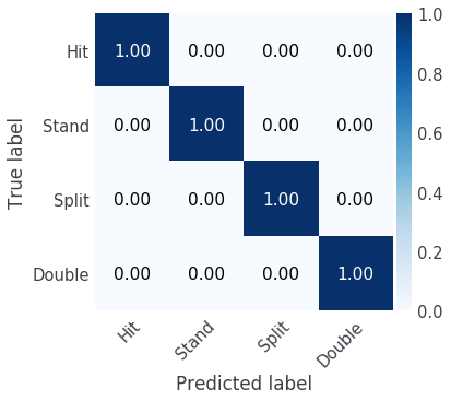
jtplot.style(context='paper', fscale=1.4, spines=False, gridlines='')
classes = list(action_to_class.keys())
plot_confusion_matrix(label.cpu(), pred.cpu(), classes=classes, normalize=True, title=' ', figsize=(6,6))
plt.show()
Normalized confusion matrix
[[1. 0. 0. 0.]
 [0. 1. 0. 0.]
 [0. 0. 1. 0.]
 [0. 0. 0. 1.]]
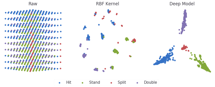
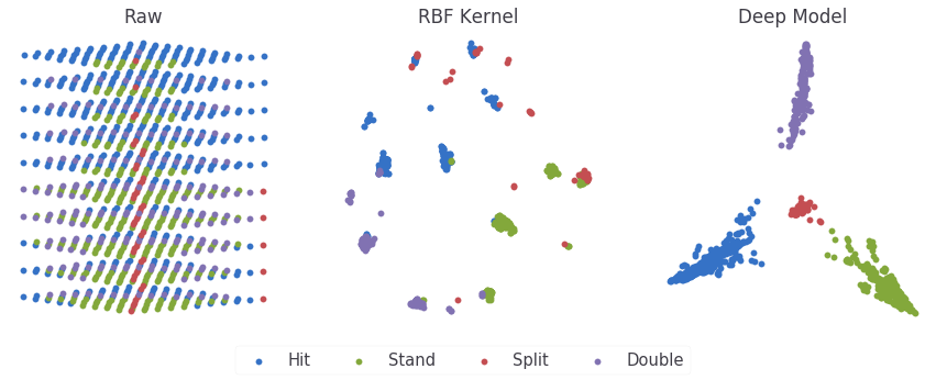
Visualization of A, RBF, and Deep Model representations
from sklearn.decomposition import PCA
a = A.cpu().detach().numpy()
pca = PCA(2)
y = pca.fit_transform(a)
l = label.cpu().detach().numpy()
p = pred.cpu().detach().numpy()
X = out.cpu().detach().numpy()
fig, ax = plt.subplots(1,3, figsize=(15,5))
ax[0].scatter(y[l==0,0], y[l==0,1], label='Hit')
ax[0].scatter(y[l==1,0], y[l==1,1], label='Stand')
ax[0].scatter(y[l==2,0], y[l==2,1], label='Split')
ax[0].scatter(y[l==3,0], y[l==3,1], label='Double')
ax[0].set_xticks([])
ax[0].set_yticks([])
ax[0].set_title('Raw')
pca = PCA(2)
y = pca.fit_transform(X)
ax[2].scatter(y[l==0,0], y[l==0,1], label='Hit')
ax[2].scatter(y[l==1,0], y[l==1,1], label='Stand')
ax[2].scatter(y[l==2,0], y[l==2,1], label='Split')
ax[2].scatter(y[l==3,0], y[l==3,1], label='Double')
ax[2].set_xticks([])
ax[2].set_yticks([])
ax[2].set_title('Deep Model')
pca = PCA(2)
y = pca.fit_transform(vals)
hit = ax[1].scatter(y[l==0,0], y[l==0,1], label='Hit')
stand = ax[1].scatter(y[l==1,0], y[l==1,1], label='Stand')
split = ax[1].scatter(y[l==2,0], y[l==2,1], label='Split')
double = ax[1].scatter(y[l==3,0], y[l==3,1], label='Double')
ax[1].set_xticks([])
ax[1].set_yticks([])
ax[1].set_title('RBF Kernel')
fig.legend(['Hit','Stand','Split','Double'], bbox_to_anchor=[0.39, 0.05],  loc='center', ncol=4)
plt.show()
Charlie Lehman
PhD Student
My research interests include robustness and explainability of deep vision models.